Sparklines in Apache Spark dataframes

As readers of this blog will know I’m a huge advocate of data visualisation techniques and an admirer of the work of Edward Tufte.

In a previous blog post we looked at how to add sparklines to a pandas DataFrame and view this in a Jupyter notebook.

I really like Pandas and with Dask it is possible to operate on larger volumes of data, however there are occasions where we might have to deal with “Big Data” volumes and for this purpose Apache spark is a better fit. In this post we examine how we could visualise a sparkline via Apache Spark using the pyspark library from python.

Firstly we want a development environment. Whilst jupyter notebooks is excellent for interactive data analysis and data science operations using python and pandas in this post we will take a look at Apache Zeppelin. Zeppelin is a very similar to jupyter notebook but offers support for python, scala and multiple interpreters.

In this exercise we will first create a new data frame

%pyspark
from pyspark.sql import *
from pyspark.sql.functions import udf, array
from datetime import datetime as Date
from pyspark.sql.types import StringType
sqlContext = SQLContext(sc)

data = [
[10,'Direct Sales',Date(2019,1,1)],
[12,'Direct Sales',Date(2019,1,2)],
[11,'Direct Sales',Date(2019,1,3)],
[15,'Direct Sales',Date(2019,1,4)],
[12,'Direct Sales',Date(2019,1,5)],
[20,'Online Sales',Date(2019,1,1)],
[25,'Online Sales',Date(2019,1,2)],
[22,'Online Sales',Date(2019,1,3)],
[30,'Online Sales',Date(2019,1,4)],
[23,'Online Sales',Date(2019,1,5)],
]

df = sqlContext.createDataFrame(data , ['Revenue','Department','Date'])

The code above will create a dataframe with 10 rows and 3 columns. This sample data is simulating 5 dates and the sales in 2 different departments.

In terms of viewing a chart we want to pivot the data, note how the syntax of the pyspark  pivot is 3 function calls and not as easy to read as the equivalent pandas pivot or pivot_table function.

df = df.groupBy("Department").pivot("Date").sum("Revenue")

Having flattened the data into 2 rows we want to add another column called “Trend” which contains the sparkline, however first we need to create the function which will draw the line.

To draw the line we will use matplotlib. Note however the function is virtually identical to the code we used for pandas.

def sparkline(data, figsize=(4, 0.25), **kwargs):
    """
    creates a sparkline
    """
    from matplotlib import pyplot as plt
    import base64
    from io import BytesIO

    data = list(data)

    *_, ax = plt.subplots(1, 1, figsize=figsize, **kwargs)
    ax.plot(data)
    ax.fill_between(range(len(data)), data, len(data)*[min(data)], alpha=0.1)
    ax.set_axis_off()

    img = BytesIO()
    plt.savefig(img)
    plt.close()
    return '%html <img src="image/png;base64, {}" />'.format(base64.b64encode(img.getvalue()).decode())

Note how the function above is effectively the same as the one we used in a previous post apart from the %html part. This string is used by the zeppelin notebook to ensure that our base64 encoded string is displayed in the notebook as HTML.

 

Next we will create a UDF and add a columns to the dataframe before finally exposing the dataframe as a table so we issue straight sql against it

pivot_udf = udf(lambda arr: sparkline(arr), StringType())

df = df.withColumn("Trend",pivot_udf(array([col for col in df.columns if col != 'Department'])))
df.registerTempTable("df")

In the lines of code above we use withColumn and pass the columns which contain the numerical data to the UDF. (The row contains Department and 5 numeric fields for each date, since the Department is a text value we do not want to pass this, hence the list comprehension used to build the array)

Finally we can view the data using a straight select statement. Note in this case the pivoted column names as dates which contain a space hence the use of backticks around the field names

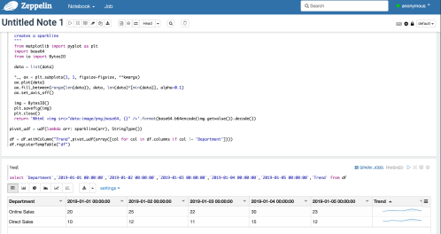
Sparkline produced using pyspark and apache Zeppelin